NUMERICAL EXPERIMENTS FOR STOCHASTIC ALGORITHMS FOR INTERWEAVE AND UNDERLAY COGNITIVE RADIOS WITH IMPERFECT CSI AND PROBABILISTIC INTERFERENCE CONSTRAINTS

This document provides numerical results that support the theoretical findings in [1].

[1] A. G. Marques, G. B. Giannakis, L. M. Lopez-Ramos, and J. Ramos, "Interweave and Underlay Cognitive Radios under Probability-of-Interference Constraints", IEEE J. Sel. Areas in Commun. (submitted 2012).

Matlab codes implementing the algorithms developed in [1] can be found here. These codes have been used to run the numerical examples presented in [1] and the ones presented in the present document. To run the codes, download them in the same folder and run the file main.m. The codes are put online to facilitate the purpose of non-commercial dissemination of scientific work. Please cite [1] and this webpage if you use our codes. Last but not least, the codes were not optimized to reduce the simulation time. If you use them and come up with a faster implementation, please let us know by mail and we will update them.

Test case I.A:

Interweave paradigm and long-term interference constraints (scheme S5). Setup I (the one in Tables I and II).

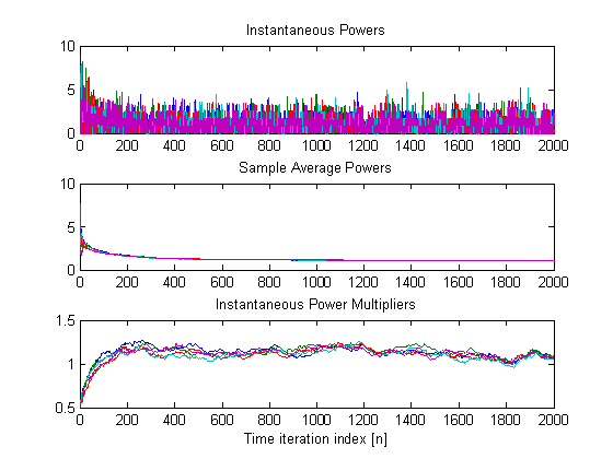
Time-trajectories of instantaneous sample average power and estimates of the power multipliers

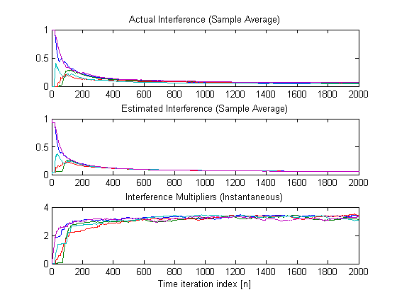
Time-trajectories of sample average interference and estimates of the interference multipliers

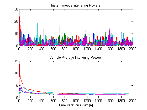
Time-trajectories of instantaneous and sample average of interfering power at the PUs

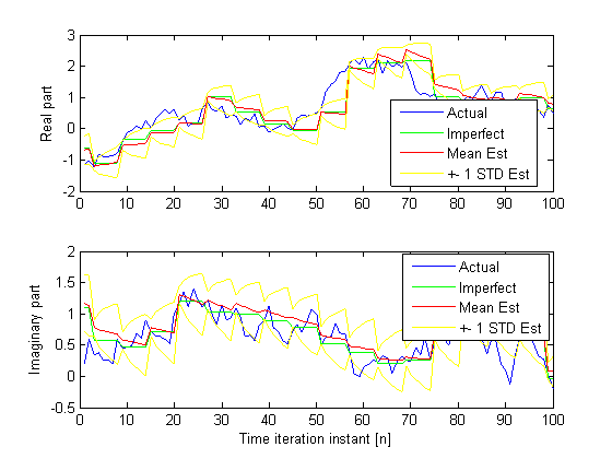
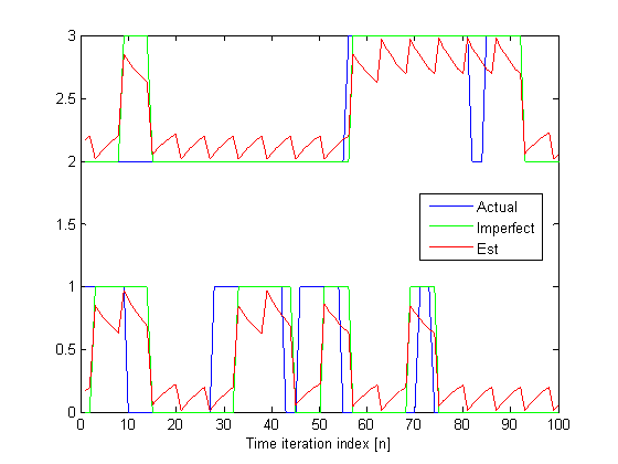
Stochastic Estimation/Belief state of the primary CSI

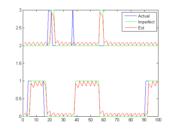
Activity of the Pus 1 and 2. To facilitate visualization only 100 instants are plotted. Moreover, the values of PU 1 are biased (adding 2) so that they do not overlap with those of PU 2.

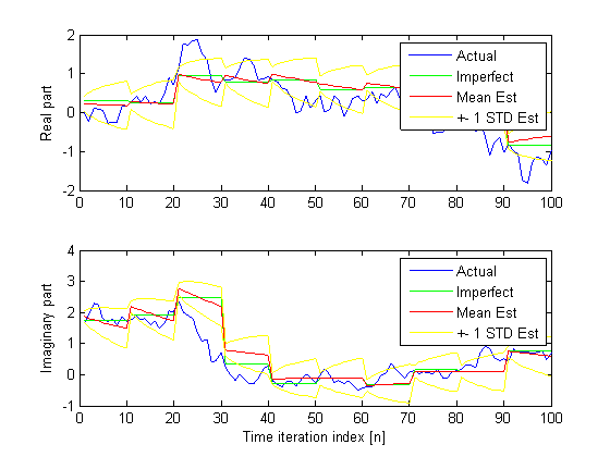
Analog (complex) gain of the CR to PU channel. The yellow lines represent the 67% confidence interval of the estimation.

Test case I.B:

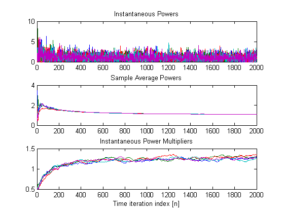
Underlay paradigm and long-term interference constraints (scheme S5). Setup I (the one in Tables I and II).

Time-trajectories of instantaneous sample average power and estimates of the power multipliers

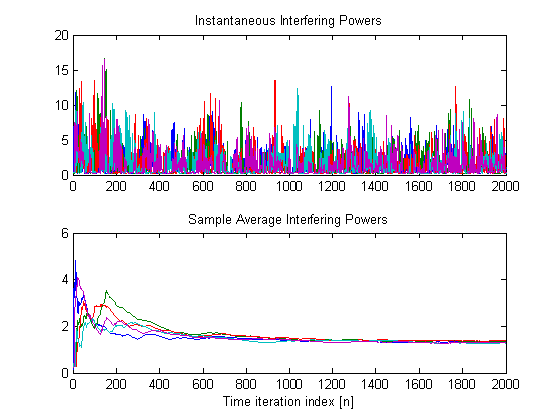
Time-trajectories of instantaneous and sample average of interfering power at the PUs

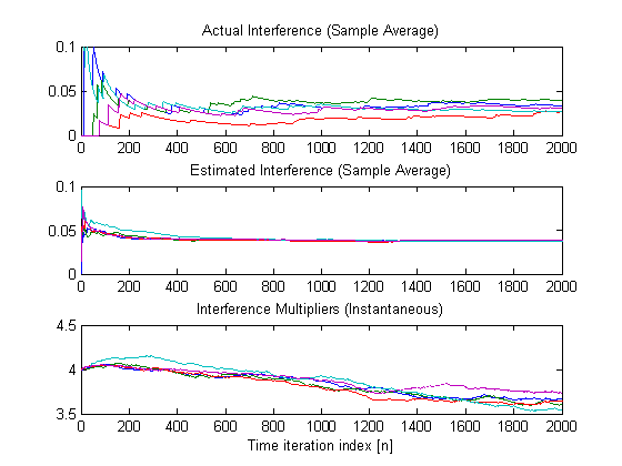
For the selected stepsize (0.1) and initialization, the interference multipliers do not converge in 2000 (see above). Expanding the time horizon we observe that “convergence” indeed occurs (see below).

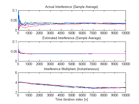
Time-trajectories of sample average interference and estimates of the interference multipliers

Stochastic Estimation/Belief state of the primary CSI (see previous test case)

Test case I.C:

Interweave paradigm and long-term interference constraints (scheme S5). Setup II (the one in Tables III and IV).

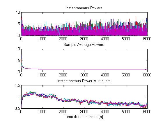
Time-trajectories of instantaneous sample average power and estimates of the power multipliers

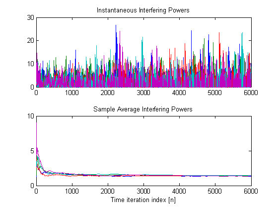
Time-trajectories of instantaneous and sample average of interfering power at the PUs

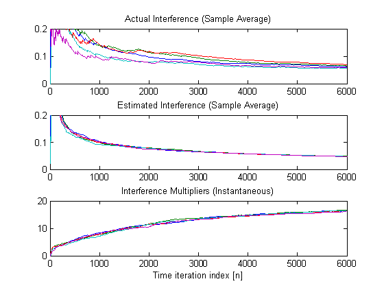
Time-trajectories of sample average interference and estimates of the interference multipliers

Stochastic Estimation/Belief state of the primary CSI

Activity of the Pus 1 and 2. To facilitate visualization only 100 instants are plotted. Moreover, the values of PU 1 are biased (adding 2) so that they do not overlap with those of PU 2.

Analog (complex) gain of the CR to PU channel. The yellow lines represent the 67% confidence interval of the estimation.

Test case II.A:

Interweave paradigm and long-term interference constraints. The setup is basically the same than in Test case 1, but here we will:

1) Change the stepsize online and see the effect on the resource allocation. We change the stepsize of the power multiplier at time n=5000.

The most important figure in this case is:

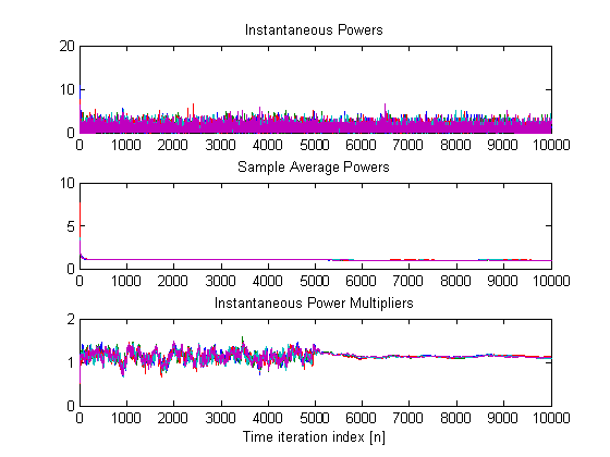
We observe how the fact of considering a much smaller stepsize, makes the hovering around the optimal value of the multiplier is much smaller (see third subplot). Moreover, we also observe that such a change does not affect the feasibility of the algorithm (second plot).

2) Online modification of the statistics (average SNR) of the channel of some of the secondary users (from 9 to 4.5). The average SNR is changed at time instant n=5000.

The most important figure in this case is:

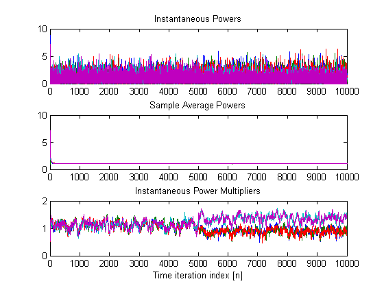
We clearly observe that before n=5000 all users were behaving similarly and that after n=5000 two different behaviors are observed (see third subplot). Specifically, users with worse channel conditions (average SNR of 4.5) have a small Lagrange multiplier and users with better channel conditions (average SNR of 9) have a larger multiplier. This way, the algorithm is able to effect fairness. Clearly, if the instantaneous realization of a good user and a bad user is the same, then the bad user will be the one accessing the channel (cf. equation for optimum scheduling).

3) Online modification of the interference requirement of the first PU (from 4% to 5%). The requirement is changed at time instant n=5000.

The most important figure in this case is:

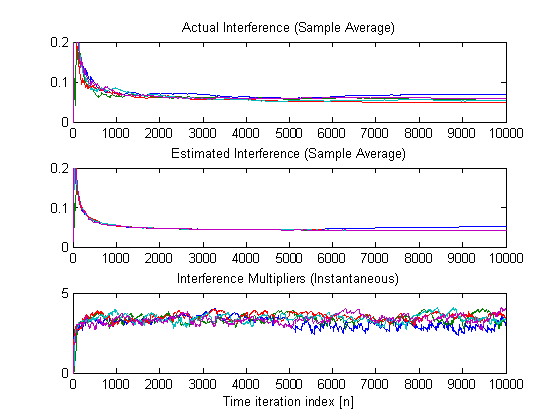
We observe that before n=5000, the value of all multipliers is basically the same and the value of the interference is the same to. However, after n=5000, we observe that the values of the first PU (blue line) start to diverge. Since more interference is allowed for that PU, its multiplier becomes smaller. Moreover, we also observe that the values of achieved interference (both estimated and actual) are higher for that user (full convergence did not take place at n=10000).

Both 2) and 3) confirm that the algorithms are able to track changes.